Probability inequalities

In probability and statistics, we often want to know how likely a random variable is to be far from its expectation. Computing this exactly requires knowing the full distribution. In many problems, especially in statistical learning theory and machine learning, we either do not know the full distribution or it is too complicated to work with directly.

The bounds in this post fall into two groups. Tail and concentration inequalities bound the probability that a random variable deviates from its mean, and the union bound, Markov’s inequality, Chebyshev’s inequality, the Chernoff bound, and Hoeffding’s inequality are examples of this. We also have expectation inequalities, such as the Cauchy–Schwarz and Jensen inequalities. These underpin many arguments in probability and statistics (for instance, the Cauchy–Schwarz inequality is the key step in the proof of the Cramér–Rao lower bound).

Union bound

The union bound (also called Boole’s inequality) is the simplest probability inequality. It gives an upper bound on the probability that at least one event in a collection occurs: the probability of the union is at most the sum of the individual probabilities.

Proof. By induction on $n$. For $n = 1$ the statement is trivial. Suppose the bound holds for $n$. Using $\mathbb{P}(A \cup B) = \mathbb{P}(A) + \mathbb{P}(B) - \mathbb{P}(A \cap B) \leq \mathbb{P}(A) + \mathbb{P}(B)$:

$$ \mathbb{P}\!\left(\bigcup_{i=1}^{n+1} E_i\right) \leq \mathbb{P}\!\left(\bigcup_{i=1}^n E_i\right) + \mathbb{P}(E_{n+1}) \leq \sum_{i=1}^{n+1} \mathbb{P}(E_i). \quad\square $$

The bound is tight when the events are mutually exclusive, and loose when they overlap heavily. Despite its simplicity, the union bound is the standard first step in arguments that control the probability of “anything going wrong” when there are many potential failure modes. If each of $n$ events has probability at most $\delta/n$, then the probability that any of them occurs is at most $\delta$.

Markov’s inequality

Markov’s inequality is the most fundamental tail bound, and essentially every other inequality in this post is a consequence of it. It says that a non-negative random variable is unlikely to be much larger than its mean: if the average value is small, the variable cannot be large too often, or the average would be dragged up.

Proof. Since $Z \geq 0$, we have $Z/t \geq \mathbf{1}\{Z \geq t\}$: if $Z \geq t$ then $Z/t \geq 1$; if $Z < t$ then $Z/t \geq 0$. Taking expectations:

$$ \mathbb{P}(Z \geq t) = \mathbb{E}[\mathbf{1}\{Z \geq t\}] \leq \mathbb{E}\!\left[\frac{Z}{t}\right] = \frac{\mathbb{E}[Z]}{t}. \quad\square $$

Markov’s inequality uses only the mean and the non-negativity of $Z$. The price of this generality is that the bound is often very loose. But its real power lies in the fact that applying it to a carefully chosen transformation of the original variable produces much tighter results — as we see next.

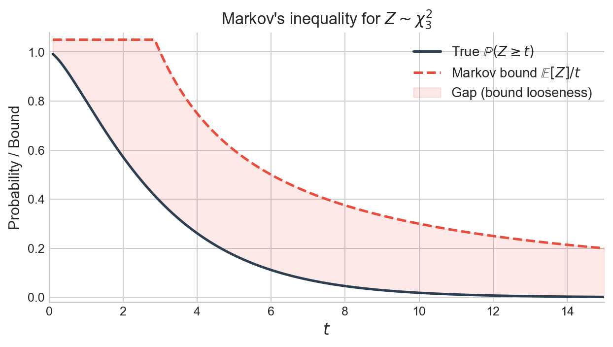
Figure 1. Markov’s inequality for a $\chi^2_3$ random variable. The solid curve is the true tail probability $\mathbb{P}(Z \geq t)$; the dashed curve is the Markov bound $\mathbb{E}[Z]/t = 3/t$. The bound is valid for all $t > 0$ but increasingly loose in the tail.

Chebyshev’s inequality

If we also know the variance, we can do better by applying Markov’s inequality to the squared deviation $(Z - \mathbb{E}[Z])^2$. This yields Chebyshev’s inequality, which bounds the probability of deviating from the mean in either direction.

Proof. The event $\{|Z - \mathbb{E}[Z]| \geq t\}$ is the same as $\{(Z - \mathbb{E}[Z])^2 \geq t^2\}$. Since $(Z - \mathbb{E}[Z])^2$ is non-negative, Markov’s inequality gives

$$ \mathbb{P}(|Z - \mathbb{E}[Z]| \geq t) = \mathbb{P}\!\left((Z - \mathbb{E}[Z])^2 \geq t^2\right) \leq \frac{\mathbb{E}[(Z - \mathbb{E}[Z])^2]}{t^2} = \frac{\text{Var}(Z)}{t^2}. \quad\square $$

Chebyshev’s inequality already has powerful consequences. If $X_1, \ldots, X_n$ are i.i.d. with mean $\mu$ and finite variance $\sigma^2$, then $\text{Var}(\bar X_n) = \sigma^2/n$, so

$$ \mathbb{P}(|\bar X_n - \mu| \geq \varepsilon) \leq \frac{\sigma^2}{n\varepsilon^2} \to 0, $$

which is a proof of the Weak Law of Large Numbers.

Chernoff bound

Chebyshev’s inequality improves on Markov by exploiting the second moment. The natural question is: can we use even higher-order information? The Chernoff bound answers this by leveraging the moment generating function (MGF), which encodes all moments at once.

The moment generating function of a random variable $Z$ is

$$ M_Z(\lambda) = \mathbb{E}[e^{\lambda Z}], $$

which may be finite or infinite depending on $\lambda$ and the distribution of $Z$. The key property of the MGF is that it factorises over independent sums: if $Z_1, \ldots, Z_n$ are independent, then

$$ M_{Z_1 + \cdots + Z_n}(\lambda) = \prod_{i=1}^n M_{Z_i}(\lambda). $$

This makes the Chernoff bound especially effective for sums of independent random variables.

Proof. For any $\lambda > 0$, the event $\{Z - \mathbb{E}[Z] \geq t\}$ is equivalent to $\{e^{\lambda(Z - \mathbb{E}[Z])} \geq e^{\lambda t}\}$. Since the exponential is non-negative, Markov’s inequality gives

$$ \mathbb{P}(Z - \mathbb{E}[Z] \geq t) = \mathbb{P}\!\left(e^{\lambda(Z - \mathbb{E}[Z])} \geq e^{\lambda t}\right) \leq \frac{\mathbb{E}\!\left[e^{\lambda(Z - \mathbb{E}[Z])}\right]}{e^{\lambda t}}. $$

Since $\lambda > 0$ was arbitrary (and the bound trivially holds at $\lambda = 0$), we take the infimum over $\lambda \geq 0$. $\square$

The Chernoff bound is a technique rather than a single formula: the quality of the bound depends on how well we can evaluate or bound the MGF for the specific distribution at hand. Its structural advantage is the factorisation of MGFs over independent sums: bounding the MGF of a sum reduces to bounding the MGF of each summand separately.

Hoeffding’s inequality

Hoeffding’s inequality is what the Chernoff technique delivers when the summands are bounded. It gives a exponential tail bound for averages of independent bounded random variables, and is one of the most widely used concentration inequalities in statistical learning theory.

The key ingredient is Hoeffding’s lemma, which bounds the MGF of a bounded, mean-zero random variable.

The lemma says that the MGF of a bounded, centred random variable is controlled by a Gaussian-like expression whose width depends only on the range $b - a$, not on the particular distribution of $Z$. The proof uses convexity of the exponential and a careful bounding argument; it is given in A1.

Combining Hoeffding’s lemma with the Chernoff bound gives the main result.

Proof. Write $W_i = Z_i - \mathbb{E}[Z_i]$, so $\mathbb{E}[W_i] = 0$ and $W_i \in [a_i - \mathbb{E}[Z_i],\; b_i - \mathbb{E}[Z_i]]$, a range of length $b_i - a_i$. By the Chernoff bound, for any $\lambda > 0$:

$$ \mathbb{P}\!\left(\sum_{i=1}^n W_i \geq nt\right) \leq e^{-\lambda nt}\, \prod_{i=1}^n \mathbb{E}\!\left[e^{\lambda W_i}\right]. $$

Applying Hoeffding’s lemma to each factor:

$$ \prod_{i=1}^n \mathbb{E}\!\left[e^{\lambda W_i}\right] \leq \exp\!\left(\frac{\lambda^2}{8} \sum_{i=1}^n (b_i - a_i)^2\right). $$

Write $S = \sum_{i=1}^n (b_i - a_i)^2$ and minimise over $\lambda > 0$:

$$ \inf_{\lambda > 0}\, \exp\!\left(\frac{\lambda^2 S}{8} - \lambda nt\right) = \exp\!\left(-\frac{2n^2 t^2}{S}\right), $$

attained at $\lambda^* = 4nt/S$. $\square$

By a union bound over the upper and lower tails, we also obtain the two-sided version:

$$ \mathbb{P}\!\left(\left|\frac{1}{n}\sum_{i=1}^n (Z_i - \mathbb{E}[Z_i])\right| \geq t\right) \leq 2\exp\!\left(-\frac{2nt^2}{(b-a)^2}\right). $$

Hoeffding’s inequality is useful precisely when we know only that the variables are bounded and independent — we do not need to know their individual distributions, only their ranges.

Comparing tightness

The inequalities above form a hierarchy: each uses more information about the distribution and produces a tighter bound. To see this concretely, consider $X \sim \text{Binom}(n, 1/2)$ and the tail probability $\mathbb{P}(X \geq 3n/4)$.

Markov’s inequality. Since $\mathbb{E}[X] = n/2$ and $X \geq 0$:

$$ \mathbb{P}(X \geq 3n/4) \leq \frac{n/2}{3n/4} = \frac{2}{3}. $$

This bound does not depend on $n$ at all.

Chebyshev’s inequality. Since $\text{Var}(X) = n/4$ and $3n/4 = n/2 + n/4$:

$$ \mathbb{P}(X \geq 3n/4) \leq \mathbb{P}(|X - n/2| \geq n/4) \leq \frac{n/4}{(n/4)^2} = \frac{4}{n}. $$

This decays like $1/n$ — polynomial.

Chernoff bound. The MGF of $\text{Binom}(n, 1/2)$ is $M_X(\lambda) = ((e^\lambda + 1)/2)^n$. Optimising the Chernoff bound yields

$$ \mathbb{P}(X \geq 3n/4) \leq \left(\frac{16}{27}\right)^{n/4}. $$

This decays exponentially in $n$.

Hoeffding’s inequality. Writing $X = \sum_{i=1}^n X_i$ with $X_i \sim \text{Bern}(1/2)$ independently:

$$ \mathbb{P}\!\left(\frac{1}{n}\sum_{i=1}^n X_i - \frac{1}{2} \geq \frac{1}{4}\right) \leq e^{-n/8}. $$

This also decays exponentially, though with a different constant in the exponent.

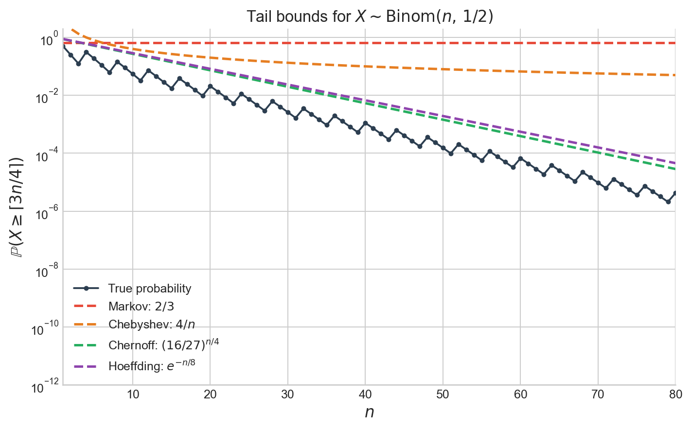
Figure 2. True tail probability $\mathbb{P}(X \geq \lceil 3n/4 \rceil)$ for $X \sim \text{Binom}(n, 1/2)$ (black) alongside the Markov, Chebyshev, Chernoff, and Hoeffding upper bounds. The Markov bound is constant; Chebyshev decays polynomially; Chernoff and Hoeffding decay exponentially.

Each step up in the hierarchy of inequalities trades generality for tightness: Markov applies to any non-negative random variable, while Hoeffding requires independence and boundedness. In exchange, Hoeffding’s exponential decay is vastly sharper than Markov’s constant bound, especially for large $n$.

Cauchy–Schwarz inequality

The Cauchy–Schwarz inequality is a fundamental inequality relating expectations of products to expectations of squares. It appears throughout probability and statistics; for instance, it is the key ingredient in the proof of the Cramér–Rao lower bound.

The intuition is the same as in linear algebra: the inner product of two vectors is bounded by the product of their norms. Here the “vectors” are random variables, the “inner product” is $\mathbb{E}[XY]$, and the “norm” is $(\mathbb{E}[X^2])^{1/2}$.

Proof. For any $s \in \mathbb{R}$, the random variable $(X - sY)^2$ is non-negative, so

$$ g(s) = \mathbb{E}[(X - sY)^2] = \mathbb{E}[X^2] - 2s\,\mathbb{E}[XY] + s^2\,\mathbb{E}[Y^2] \geq 0. $$

This is a quadratic in $s$ that is everywhere non-negative, so its discriminant must be non-positive:

$$ 4(\mathbb{E}[XY])^2 - 4\,\mathbb{E}[X^2]\,\mathbb{E}[Y^2] \leq 0. \quad\square $$

A direct consequence is the correlation bound: for any random variables $X$ and $Y$ with positive variances, $|\rho(X,Y)| \leq 1$. This follows by applying Cauchy–Schwarz to the centred variables $X - \mathbb{E}[X]$ and $Y - \mathbb{E}[Y]$.

Jensen’s inequality

Jensen’s inequality relates the expectation of a function to the function of the expectation. The direction of the inequality is determined by convexity, and the result is used throughout statistics, information theory, and optimisation.

Recall that a function $g : \mathbb{R} \to \mathbb{R}$ is convex if for all $x, y$ and all $\lambda \in [0, 1]$:

$$ g(\lambda x + (1-\lambda)y) \leq \lambda g(x) + (1-\lambda) g(y). $$

Geometrically, the chord between any two points on the graph of $g$ lies above the graph. If $g$ is twice differentiable, convexity is equivalent to $g''(x) \geq 0$ everywhere. A function is concave if $-g$ is convex.

The simplest way to remember the direction: take $g(x) = x^2$ (convex) and any random variable with $\mathbb{E}[X] = 0$. Then $g(\mathbb{E}[X]) = 0 \leq \mathbb{E}[X^2]$, which is the statement that variance is non-negative.

Proof. Since $g$ is convex, it lies above every supporting line: for any $c$, there exists a slope $a$ such that $g(x) \geq a(x - c) + g(c)$ for all $x$. Take $c = \mathbb{E}[X]$:

$$ g(X) \geq a(X - \mathbb{E}[X]) + g(\mathbb{E}[X]). $$

Taking expectations:

$$ \mathbb{E}[g(X)] \geq a \cdot \mathbb{E}[X - \mathbb{E}[X]] + g(\mathbb{E}[X]) = g(\mathbb{E}[X]). \quad\square $$

Jensen’s inequality has many standard applications:

• Variance is non-negative. $g(x) = x^2$ is convex, so $\mathbb{E}[X^2] \geq (\mathbb{E}[X])^2$.
• AM–GM inequality. $g(x) = -\log x$ is convex, so $-\log\!\left(\frac{1}{n}\sum a_i\right) \leq -\frac{1}{n}\sum \log a_i$, giving $\frac{1}{n}\sum a_i \geq (\prod a_i)^{1/n}$.
• KL divergence is non-negative. $g(x) = -\log x$ applied to the density ratio $q(X)/p(X)$ under $p$ gives $D_{\text{KL}}(p \| q) \geq 0$.
• Log-likelihood bounds. The concavity of $\log$ is what makes the evidence lower bound (ELBO) in variational inference a lower bound.

Appendix

A1: Proof of Hoeffding’s lemma

Proof. Let $Z \in [a, b]$ with $\mathbb{E}[Z] = 0$. Since $Z \in [a, b]$, we can write $Z$ as a convex combination of the endpoints:

$$ Z = \frac{b - Z}{b - a}\, a + \frac{Z - a}{b - a}\, b. $$

By convexity of $x \mapsto e^{\lambda x}$:

$$ e^{\lambda Z} \leq \frac{b - Z}{b - a}\, e^{\lambda a} + \frac{Z - a}{b - a}\, e^{\lambda b}. $$

Taking expectations and using $\mathbb{E}[Z] = 0$:

$$ \mathbb{E}[e^{\lambda Z}] \leq \frac{b}{b - a}\, e^{\lambda a} + \frac{-a}{b - a}\, e^{\lambda b}. $$

Define $\theta = -a/(b - a) \in [0, 1]$ (which lies in $[0,1]$ because $\mathbb{E}[Z] = 0$ forces $a \leq 0 \leq b$) and $h = \lambda(b - a)$. Then $\lambda a = -\theta h$ and $\lambda b = (1 - \theta)h$, so

$$ \mathbb{E}[e^{\lambda Z}] \leq (1 - \theta)\, e^{-\theta h} + \theta\, e^{(1-\theta)h} = e^{\varphi(h)}, $$

where $\varphi(h) = -\theta h + \log(1 - \theta + \theta e^h)$. It suffices to show $\varphi(h) \leq h^2/8$.

We have $\varphi(0) = 0$ and $\varphi'(0) = -\theta + \theta/(1 - \theta + \theta) = 0$. The second derivative is

$$ \varphi''(h) = \frac{\theta e^h (1 - \theta)}{(1 - \theta + \theta e^h)^2}. $$

Setting $u = \theta e^h / (1 - \theta + \theta e^h) \in (0, 1)$, we can write $\varphi''(h) = u(1 - u) \leq 1/4$. Since $\varphi(0) = 0$, $\varphi'(0) = 0$, and $\varphi''(h) \leq 1/4$ for all $h$, Taylor’s theorem with remainder gives

$$ \varphi(h) = \varphi(0) + h\,\varphi'(0) + \frac{h^2}{2}\,\varphi''(c) \leq \frac{h^2}{8} $$

for some $c$ between $0$ and $h$. Therefore $\mathbb{E}[e^{\lambda Z}] \leq e^{h^2/8} = e^{\lambda^2(b-a)^2/8}$. $\square$

Sources

Much of the material in this post is covered in the Maths of Machine Learning course at the University of Cambridge. The presentation of Chernoff and Hoeffding bounds draws on the CS229 supplemental notes listed below.

• Rajen Shah, Maths of Machine Learning, University of Cambridge lecture notes, Sections 3.1–3.2.
• John Duchi, “Hoeffding’s inequality,” CS229 supplemental lecture notes, Stanford University.

The full code for the figures is in the Jupyter notebook on GitHub.