The same formula $f(x, \theta)$ can be read in two entirely different ways. As a function of $x$ for fixed $\theta$, it is a probability model: it tells you how likely different data values are under a given parameter. As a function of $\theta$ for fixed observed $x$, it is the likelihood function: it tells you which parameter values make the observed data more or less plausible.
Most confusion about likelihood comes from mixing up what is random and what is fixed. This post explains the distinction carefully, and then follows it to its natural consequences: the log-likelihood, the score function, maximum likelihood estimation, and the population interpretation via KL divergence.
The likelihood function
Start from a parametric model $\{f(\cdot, \theta) : \theta \in \Theta\}$. For each fixed $\theta$, the function $x \mapsto f(x, \theta)$ is a density or probability mass function on the sample space: it assigns probability (or probability density) to data values.
Now suppose we observe data $x$. Define the likelihood function by
$$ L(\theta; x) = f(x, \theta), $$regarded as a function of $\theta$ for fixed $x$. The algebraic expression is identical, but the roles of the two arguments have reversed: $x$ is now held constant and $\theta$ is the variable.
Probability asks: if the parameter were $\theta$, how likely are different data values? Likelihood asks: given the data we saw, which parameter values make them more plausible?
The word “likelihood” is about relative support among parameter values. It does not assign probabilities to parameter values. If we compare the likelihood function at two parameter points and find that $L(\theta_1; x) > L(\theta_2; x)$ this can be interpreted as saying that the observed data are more consistent with $\theta_1$ than with $\theta_2$ under the model.
A common convention is to define the likelihood only up to positive proportionality: multiplying by any positive constant that does not depend on $\theta$ changes nothing about relative comparisons or the location of the maximum. We will use $L(\theta; x)$ for the observed likelihood (a deterministic function of $\theta$), and $L(\theta; X)$ for the likelihood as a random function before data are observed, random because $X$ is.
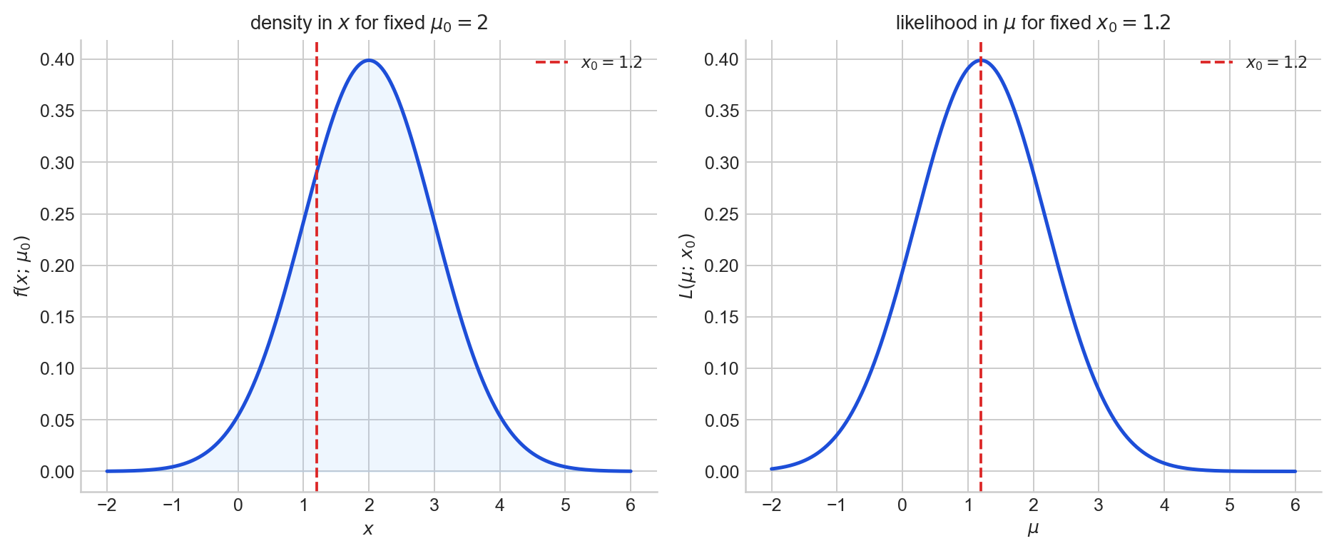
Figure 1. Left: $x \mapsto f(x; \mu_0)$ is a density in the data for fixed $\mu_0 = 2$. Right: $\mu \mapsto L(\mu; x_0) = f(x_0; \mu)$ is a likelihood curve in the parameter for fixed $x_0 = 1.2$.
Likelihood for an i.i.d. sample
If $X_1, \dots, X_n \stackrel{\text{i.i.d.}}{\sim} f(\cdot, \theta)$, then the joint density is the product of the individual densities, and the likelihood becomes
$$ L_n(\theta; x_1, \dots, x_n) = \prod_{i=1}^n f(x_i, \theta). $$Independence turns the plausibility of the whole sample into a product of per-observation plausibilities. Taking logarithms gives the log-likelihood
$$ \ell_n(\theta) = \log L_n(\theta) = \sum_{i=1}^n \log f(x_i, \theta), $$and the average log-likelihood
$$ \bar\ell_n(\theta) = \frac{1}{n} \ell_n(\theta) = \frac{1}{n} \sum_{i=1}^n \log f(x_i, \theta). $$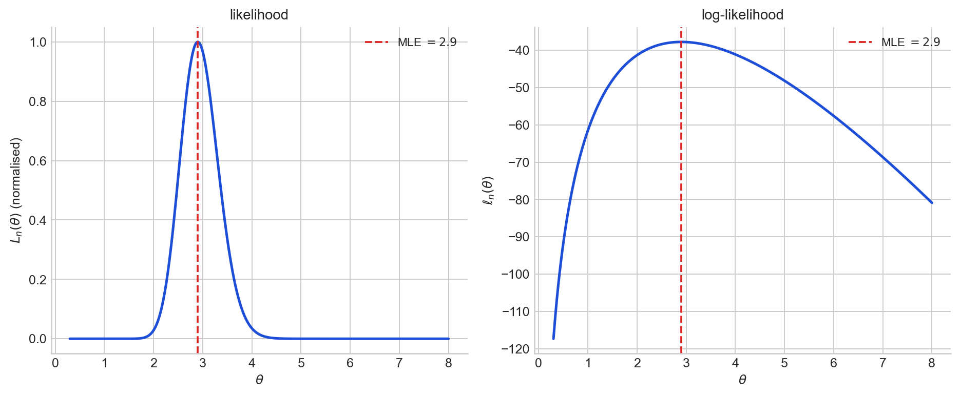
Figure 2. Left: the likelihood $L_n(\theta)$ for a single Poisson sample. Right: the log-likelihood $\ell_n(\theta)$ for the same sample. The maximiser is the same.
What is random and what is fixed?
The likelihood depends on the data, and the data are random. This makes the likelihood itself a random object, but the randomness needs to be understood precisely.
Before observing data
The random variables $X_1, \dots, X_n$ have not yet been realised. The likelihood $L_n(\theta; X_1, \dots, X_n)$ is a random function of $\theta$: for each outcome $\omega$ of the experiment, the realised data $X_1(\omega), \dots, X_n(\omega)$ produce a different likelihood function (or curve)
$$ \theta \mapsto L_n(\theta; X_1(\omega), \dots, X_n(\omega)). $$In this sense, the likelihood is a random element of a function space.
After observing data
Once the data are observed as $x_1, \dots, x_n$, the likelihood $L_n(\theta; x_1, \dots, x_n)$ is just an deterministic curve over $\Theta$, there is no randomness.
The likelihood is random only because it depends on random data. Once the data are realised, the likelihood curve itself is fixed.
The analogy with estimators is helpful. Before data, an estimator $\hat\theta(X)$ is a random variable; after data, $\hat\theta(x)$ is a number. Likewise, before data, the likelihood is a random function; after data, it is a deterministic curve.
The phrase “random curve” does not mean that the randomess comes from the parameter. It means the curve you end up with depends on which sample you happened to draw.
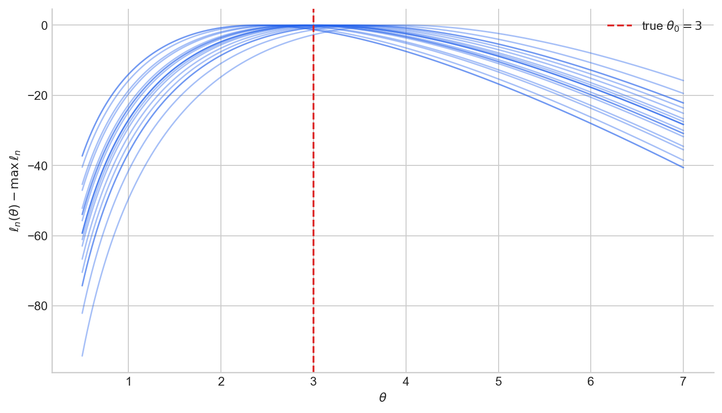
Figure 3. Twenty normalised log-likelihood curves $\ell_n(\theta) - \max_\vartheta \ell_n(\vartheta)$ from independent Poisson$(\theta_0 = 3)$ samples of size $n = 20$. Each sample produces a different curve, but they cluster around the true parameter.
Why likelihood is not a probability distribution in $\theta$
A probability density function is not just any non-negative function. It is defined relative to three things:
- a measurable space,
- a random variable taking values in that space,
- a reference measure with respect to which probabilities are computed.
Now consider a parametric model $\{f(\cdot, \theta) : \theta \in \Theta\}$. For each fixed $\theta$, the function
$$ x \mapsto f(x, \theta) $$is a density or pmf in the data variable $x$. The random variable is $X$, the space is the sample space $\mathcal{X}$, and the reference measure is whatever measure the model is defined against (Lebesgue measure if $X$ is continuous, counting measure if $X$ is discrete).
But once we observe $x$ and write
$$ \theta \mapsto L(\theta; x) = f(x, \theta), $$we are no longer looking at a density in the random variable $X$. We are looking at a function of the parameter $\theta$, on the parameter space $\Theta$. In the usual frequentist setup, the parameter $\theta$ is not a random variable; it is an unknown but fixed constant. Since there is no random variable $\theta$, there is no probability law on parameter space for $L(\theta; x)$ to be a density of.
If one does introduce a prior $\pi(\theta)$, which amounts to modelling $\theta$ as random, then the posterior density
$$ \pi(\theta \mid x) \propto L(\theta; x) \, \pi(\theta) $$is a proper density on $\Theta$ (under mild conditions). But the posterior depends on the choice of prior: the likelihood alone does not determine a distribution over $\theta$.
So the likelihood is not a probability distribution over $\theta$. It is a non-negative function on parameter space that tells us how well different parameter values explain the observed data, i.e. a function for comparing parameter values, not for assigning probabilities to them.
Maximum likelihood estimation
Given observed data $x_1, \dots, x_n$, the maximum likelihood estimator (MLE) is any value $\hat\theta$ that maximises the likelihood (or equivalently, the log-likelihood) over the parameter space:
$$ \hat\theta \in \arg\max_{\theta \in \Theta} L_n(\theta; x_1, \dots, x_n) = \arg\max_{\theta \in \Theta} \ell_n(\theta; x_1, \dots, x_n). $$The equivalence holds because $\log$ is strictly increasing, so it preserves the location of the maximum. Intuitively, the MLE is the parameter value under which the observed sample is most plausible according to the model.
Before the data are observed, $\hat\theta = \hat\theta(X_1, \dots, X_n)$ is a random variable, it depends on the random sample. After the data are observed, it is a number. This is the same before-versus-after distinction that applies to the likelihood itself.
The MLE need not exist (the log-likelihood may increase without bound), need not be unique (there may be multiple global maxima), and may lie on the boundary of $\Theta$. When $\Theta$ is open and $\ell_n$ is differentiable, an interior MLE satisfies the score equation $S_n(\hat\theta) = 0$ and we must ensure it is a global maximum.
Worked example: Poisson
Suppose $X_1, \dots, X_n \stackrel{\text{i.i.d.}}{\sim} \text{Poisson}(\theta)$, $\theta > 0$. The likelihood is
$$ L_n(\theta) = \prod_{i=1}^n \frac{e^{-\theta} \theta^{x_i}}{x_i!} \propto e^{-n\theta} \theta^{\sum x_i}. $$The log-likelihood, up to an additive constant not depending on $\theta$, is
$$ \ell_n(\theta) = -n\theta + \left(\sum_{i=1}^n x_i\right) \log\theta + C. $$The parameter space is $\Theta = (0, \infty)$, which is open, so if a maximum exists in the interior it must satisfy the score equation. Differentiating:
$$ \ell_n'(\theta) = -n + \frac{\sum_{i=1}^n x_i}{\theta}. $$Setting $\ell_n'(\theta) = 0$ gives $\hat\theta = \bar X$. To confirm this is a maximum rather than a minimum or saddle point, compute the second derivative:
$$ \ell_n''(\theta) = -\frac{\sum_{i=1}^n x_i}{\theta^2}. $$When the sample is not all zeros, $\sum x_i > 0$ and so $\ell_n''(\theta) < 0$ for all $\theta > 0$: the log-likelihood is strictly concave, and the unique stationary point $\hat\theta = \bar X$ is the global maximum. (If all observations are zero, then $\ell_n(\theta) = -n\theta + C$, which is strictly decreasing on $(0, \infty)$: the supremum is approached as $\theta \to 0^+$ but is not attained in the open parameter space.)
Expected log-likelihood and KL divergence
The average log-likelihood
$$ \bar\ell_n(\theta) = \frac{1}{n} \sum_{i=1}^n \log f(X_i, \theta) $$is a sample average. By the law of large numbers, for each fixed $\theta$ it converges to a population quantity:
$$ \bar\ell_n(\theta) \to \mathbb{E}_{\theta_0}[\log f(X, \theta)] =: \ell(\theta). $$The function $\ell(\theta)$ is the expected log-likelihood under the true model. It is deterministic, it depends on the unknown $\theta_0$, and we never observe it directly. But it is the population target that the empirical curve $\bar\ell_n(\theta)$ approximates.
The MLE maximises $\bar\ell_n(\theta)$, which is a sample approximation to the population criterion $\ell(\theta)$. But what does maximising $\ell(\theta)$ actually achieve?
Cross-entropy and KL divergence
The expected log-likelihood $\ell(\theta) = \mathbb{E}_{\theta_0}[\log f(X, \theta)]$ is the negative of the cross-entropy of the true distribution $P_{\theta_0}$ and the model $P_\theta$. In information theory, cross-entropy measures the average number of bits/nats needed to encode data from $P_{\theta_0}$ using a code optimised for $P_\theta$. The KL divergence from $P_{\theta_0}$ to $P_\theta$ is defined as
$$ \text{KL}(P_{\theta_0} \| P_\theta) = \mathbb{E}_{\theta_0}\!\left[\log \frac{f(X, \theta_0)}{f(X, \theta)}\right]. $$It measures the additional cost of using $P_\theta$ instead of $P_{\theta_0}$: the cross-entropy of $P_{\theta_0}$ and $P_\theta$ minus the entropy of $P_{\theta_0}$ itself. Since the entropy of $P_{\theta_0}$ does not depend on $\theta$, we can write
$$ \ell(\theta) - \ell(\theta_0) = \mathbb{E}_{\theta_0}\!\left[\log \frac{f(X, \theta)}{f(X, \theta_0)}\right] = -\text{KL}(P_{\theta_0} \| P_\theta). $$The KL divergence satisfies $\text{KL}(P_{\theta_0} \| P_\theta) \geq 0$, with equality if and only if $P_\theta = P_{\theta_0}$. Therefore $\ell(\theta) \leq \ell(\theta_0)$ for all $\theta$, with equality exactly when the model matches the truth. Note that KL divergence is not symmetric: $\text{KL}(P \| Q) \neq \text{KL}(Q \| P)$ in general, it is not a metric.
Putting this together, maximising $\ell(\theta)$ over $\theta$ is equivalent to minimising $\text{KL}(P_{\theta_0} \| P_\theta)$, i.e. choosing the model distribution closest to the truth in the sense of KL divergence.
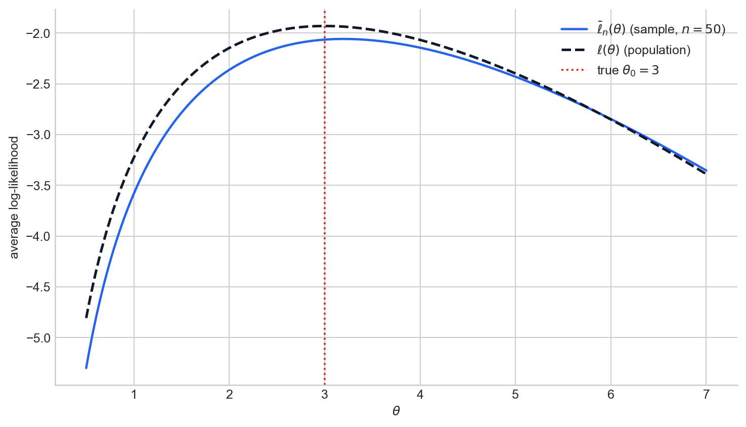
Figure 4. The average log-likelihood $\bar\ell_n(\theta)$ for one Poisson sample (solid) alongside the expected log-likelihood $\ell(\theta)$ (dashed). The sample criterion approximates the population target, and the population target is maximised at the true $\theta_0$.
The score function
The score function is the derivative of the log-likelihood with respect to the parameter:
$$ S_n(\theta) = \frac{d}{d\theta} \ell_n(\theta). $$In higher dimensions, the score is the gradient $S_n(\theta) = \nabla_\theta \ell_n(\theta)$.
The score tells you which way the log-likelihood is sloping at a given parameter value: positive score means the log-likelihood is locally increasing, negative means it is locally decreasing, and zero means you are at a stationary point.
Derivatives are taken with respect to the parameter $\theta$, not the data. The data are fixed once observed; it is $\theta$ that varies.
For the Poisson model, the score for a single observation is
$$ S(\theta) = \frac{d}{d\theta} \log f(X, \theta) = \frac{d}{d\theta}\bigl(-\theta + X\log\theta\bigr) = -1 + \frac{X}{\theta}, $$and for the full sample:
$$ S_n(\theta) = -n + \frac{\sum_{i=1}^n X_i}{\theta}. $$Setting $S_n(\theta) = 0$ recovers the MLE $\hat\theta = \bar X$.
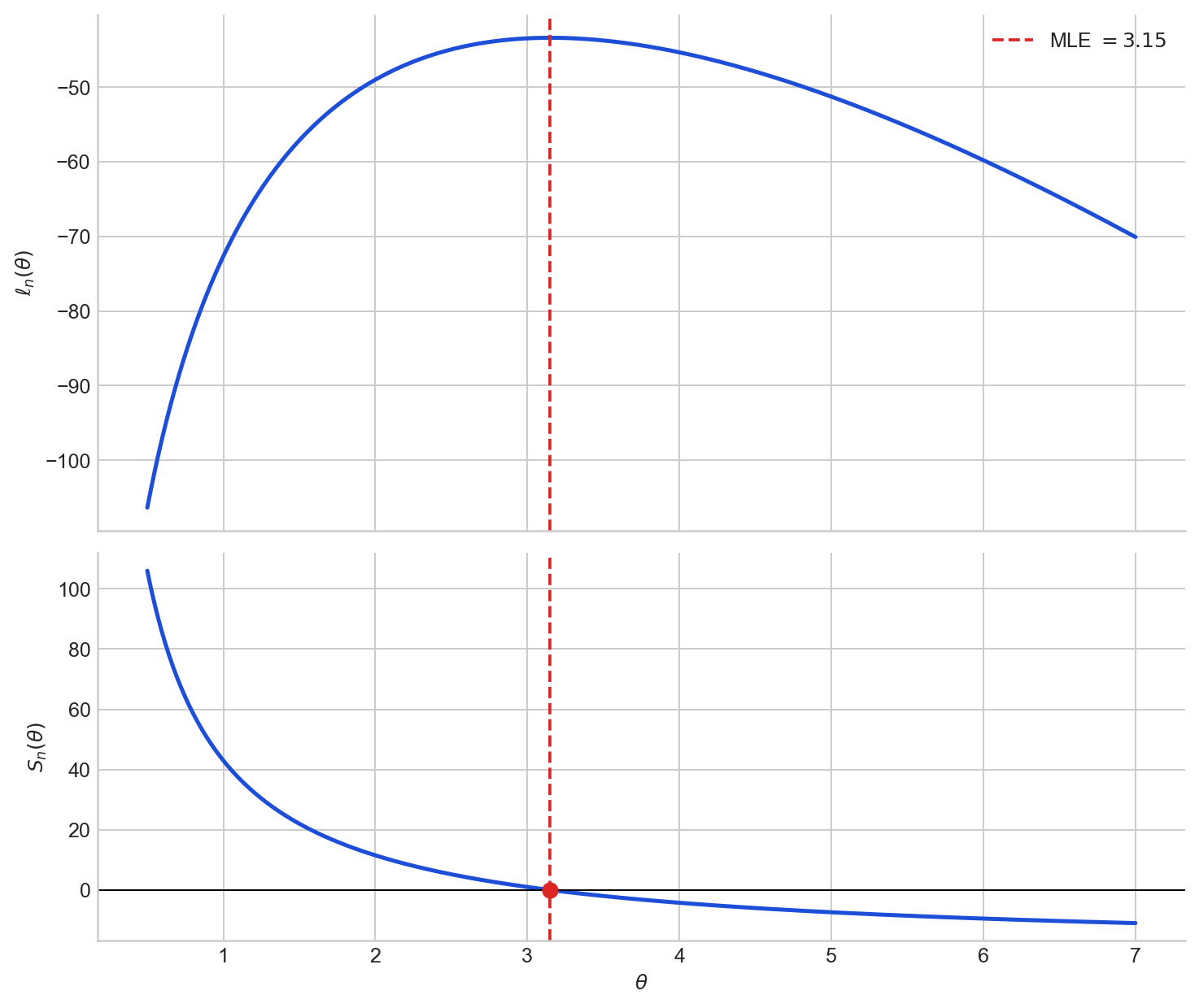
Figure 5. Top: the log-likelihood $\ell_n(\theta)$ for one Poisson sample. Bottom: the score $S_n(\theta)$ for the same sample. The score crosses zero at the MLE, where the log-likelihood reaches its maximum.
Expected score is zero
Under regularity conditions that allow differentiation under the integral sign, the expected score at the true parameter is zero:
$$ \mathbb{E}_\theta[S(\theta)] = \int \frac{\partial}{\partial\theta} \log f(x, \theta) \cdot f(x, \theta)\, dx = \int \frac{\partial}{\partial\theta} f(x, \theta)\, dx = \frac{\partial}{\partial\theta} \int f(x, \theta)\, dx = \frac{\partial}{\partial\theta}(1) = 0. $$This is an important structural property. At the true parameter, the log-likelihood has no systematic first-order tilt. Different samples produce scores that are sometimes positive and sometimes negative at $\theta_0$, but on average they balance out.
For the Poisson model, this is easy to verify directly. The score for one observation is $S(\theta) = -1 + X/\theta$. Since $\mathbb{E}_\theta(X) = \theta$:
$$ \mathbb{E}_\theta[S(\theta)] = -1 + \frac{\mathbb{E}_\theta(X)}{\theta} = -1 + \frac{\theta}{\theta} = 0. $$Sources
The material in this post draws on the likelihood inference chapter of the Principles of Statistics course at the University of Cambridge.
- Rajen Shah, Principles of Statistics, University of Cambridge lecture notes, Section 1.1.
- George Casella and Roger L. Berger, Statistical Inference, 2nd edition, Sections 6.3 and 7.2.
- “Why isn’t the likelihood function a probability density function?”, MathOverflow.
The full code for all figures is in the Jupyter notebook on GitHub.