Fisher information and the Cramér–Rao lower bound

The shape of the log-likelihood near its maximum tells you something fundamental about estimation. A sharply peaked log-likelihood means the data strongly constrain the parameter; a flat one means many parameter values are about equally compatible with what was observed.

In the previous post, we introduced the likelihood, the log-likelihood, and the score, and saw that the MLE maximises the likelihood. This post takes up the natural next question: how precisely can we estimate the parameter? Fisher information is the quantity that answers this, and the Cramér–Rao lower bound is the conclusion it leads to.

Fisher information

Scalar case

Let $X \sim f(\cdot, \theta)$ with scalar parameter $\theta \in \Theta \subseteq \mathbb{R}$. Recall that the score for a single observation is

$$ S(\theta) = \frac{\partial}{\partial\theta} \log f(X, \theta), $$

and that the expected score is zero: $\mathbb{E}_\theta[S(\theta)] = 0$. The Fisher information is the variance of the score:

$$ I(\theta) = \mathbb{E}_\theta\!\left[S(\theta)^2\right] = \text{Var}_\theta(S(\theta)). $$

Under regularity conditions that allow differentiation under the integral, there is an equivalent and often more convenient form:

$$ I(\theta) = -\mathbb{E}_\theta\!\left[\frac{\partial^2}{\partial\theta^2} \log f(X, \theta)\right]. $$

This is the expected negative curvature of the log-likelihood. Both expressions give the same number, but they offer different intuitions. The first says Fisher information is the spread of the score; the second says it is the average sharpness of the log-likelihood.

This definition is for one observation. For i.i.d. data $X_1, \dots, X_n$, Fisher information scales linearly:

$$ I_n(\theta) = n\, I_1(\theta). $$

Multivariate case

When $\theta \in \mathbb{R}^p$, the score becomes a vector $S(\theta) = \nabla_\theta \log f(X, \theta)$, and Fisher information becomes a $p \times p$ matrix:

$$ I(\theta) = \mathbb{E}_\theta\!\left[S(\theta)\, S(\theta)^\top\right]. $$

Under regularity conditions:

$$ I(\theta) = -\mathbb{E}_\theta\!\left[\nabla^2_\theta \log f(X, \theta)\right]. $$

In higher dimensions, the Fisher information matrix encodes directional structure of parameter undertainty. The data may be very informative about one combination of parameters and much less informative about another. For i.i.d. data, additivity still holds: $I_n(\theta) = n\, I_1(\theta)$.

The equivalence of the two forms of Fisher information is proved in A1, and the additivity under i.i.d. sampling in A2.

What Fisher information measures

Fisher information measures the sensitivity of the statistical model to small changes in the parameter.

If changing $\theta$ slightly causes the distribution $f(\cdot, \theta)$ to change a lot, then data drawn from the model should be informative about $\theta$. If changing $\theta$ barely changes the distribution, the data cannot tell you much about where $\theta$ is.

This sensitivity has two equivalent readings:

• Variance of the score. If the score $S(\theta)$ varies a lot across different samples, the model is responding strongly to the data at that parameter value.
• Expected negative curvature. If the log-likelihood is sharply curved on average, nearby parameter values are easy to distinguish from $\theta$ itself.

The second interpretation is especially geometric, and motivates the next section.

Why curvature matters

The log-likelihood is a random curve, and the MLE is its maximiser. The shape of that curve near its maximum should affect how much the estimator varies from sample to sample.

If the log-likelihood is sharply peaked, the MLE is tightly constrained: moving $\theta$ slightly away from the maximum causes a steep drop in log-likelihood, so different samples tend to produce similar maximisers. If the log-likelihood is flat, many parameter values achieve nearly the same likelihood, and the MLE varies more across repeated samples.

A sharper log-likelihood means more local information about the parameter, and lower estimator variance.

To make this visual, consider the Gaussian location model with known variance:

$$ X_1, \dots, X_n \sim N(\theta, \sigma^2), $$

with true parameter $\theta_0 = 0$. The log-likelihood is

$$ \ell_n(\theta) = -\frac{1}{2\sigma^2} \sum_{i=1}^n (X_i - \theta)^2 + C, $$

so its curvature is constant:

$$ \ell_n''(\theta) = -\frac{n}{\sigma^2}. $$

Smaller $\sigma^2$ means a more negative second derivative, i.e. sharper curvature. The MLE is $\hat\theta = \bar{X}$, with variance $\text{Var}(\hat\theta) = \sigma^2 / n$.

Suppose we draw $m=10$ independent samples each of size $n=20$ and plot the sample log-likelihood $\ell_n(\theta)$. Red dots mark the MLE $\hat\theta = \bar{X}$ on each curve.

When the variance is smaller (left), the log-likelihood is more sharply curved and the MLEs cluster more tightly. When the variance is larger (right), the log-likelihood is flatter and the MLEs are more spread out.

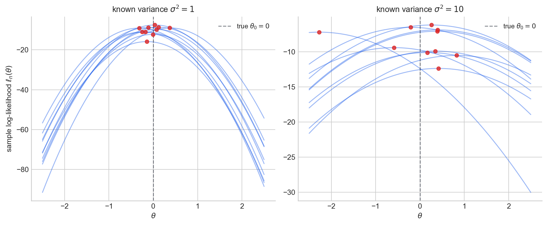
Figure 1. Sample log-likelihood $\ell_n(\theta)$ for $m = 10$ independent samples of size $n = 20$ from Gaussian location models with known variance $\sigma_1^2 = 1$ (left) and $\sigma_2^2 = 10$ (right), true mean $\theta_0 = 0$.

From observed curvature to Fisher information

The figure shows realised log-likelihood curves from random samples. Fisher information is not the curvature of any single realised curve. It is the expected negative curvature:

$$ I(\theta) = -\mathbb{E}_\theta\!\left[\frac{\partial^2}{\partial\theta^2} \log f(X, \theta)\right]. $$

Fisher information is the average local sharpness that the model tends to produce at parameter value $\theta$. The distinction matters:

• Observed curvature depends on the particular sample. It is different for each dataset.
• Fisher information is a property of the model. It averages curvature over all possible data the model could generate.

In practice, one often also uses the observed information $J(\hat\theta) = -\ell_n''(\hat\theta)$, the curvature of the realised log-likelihood evaluated at the MLE. The comparison between the observed information and the expected information remains an active and ongoing area of research and debate, but we do not discuss it here.

Information adds for i.i.d. samples

For i.i.d. observations, the log-likelihood is a sum of per-observation contributions, and the score adds accordingly:

$$ S_n(\theta) = \sum_{i=1}^n S_i(\theta), $$

where $S_i(\theta) = \frac{\partial}{\partial\theta} \log f(X_i, \theta)$. Since the $S_i$ are independent and mean-zero, the variance of the sum is the sum of the variances:

$$ I_n(\theta) = \text{Var}_\theta(S_n(\theta)) = \sum_{i=1}^n \text{Var}_\theta(S_i(\theta)) = n\, I_1(\theta). $$

Independent observations contribute independent pieces of evidence about the parameter, so information accumulates linearly.

This is one reason why variances of efficient estimators typically scale like $1/n$: information grows linearly with sample size, so uncertainty shrinks at the same rate. The proof in the multivariate case is given in A2.

The Cramér–Rao lower bound

This is a lower bound on the variance of any unbiased estimator. No matter how well an estimator is constructed, if it is unbiased then its variance cannot ne less than the reciprocal of the Fisher information. The proof uses the Cauchy–Schwarz inequality applied to the covariance between the estimator and the score, exhitbited in A3.

More general forms

We have a bound on the an estimator of a function of the parameter. If $T$ is an unbiased estimator of $g(\theta)$, then

$$ \text{Var}_\theta(T) \geq \frac{(g'(\theta))^2}{I_n(\theta)}. $$

In higher dimensions with $\theta \in \mathbb{R}^p$, the bound takes a matrix form. For any unbiased estimator $\hat\theta$ of $\theta$,

$$ \text{Cov}_\theta(\hat\theta) \succeq I_n(\theta)^{-1}, $$

meaning the difference $\text{Cov}_\theta(\hat\theta) - I_n(\theta)^{-1}$ is positive semi-definite. The inverse Fisher information matrix plays the role of the canonical covariance lower bound. The proof is in A4.

Intuition behind Cramér–Rao

If the likelihood is flat around $\theta$, many nearby parameter values produce similar likelihoods. The data cannot effectively distinguish between them, so no unbiased estimator can concentrate tightly around the truth. If the likelihood is sharp, nearby parameter values produce noticeably different likelihoods, and lower variance becomes possible.

The Cramér–Rao bound says that distinguishability (quantified by the Fisher information) sets a floor on what estimator variance is fundamentally achievable. Whether the bound is achievable depends on the model.

Achieving the bound

If an unbiased estimator achieves the Cramér–Rao lower bound, it must have the smallest possible variance among all unbiased estimators. It is a uniformly minimum-variance unbiased estimator (UMVUE).

It is worth noting that unbiasedness is itself a restriction. Some biased estimators can achieve lower mean squared error by trading a bias for a reduction in variance. But within the unbiased class, the CRLB is the definitive benchmark. The condition under which equality holds is stated in A5.

Worked example: Bernoulli model

Let $X_1, \dots, X_n \stackrel{\text{i.i.d.}}{\sim} \text{Bern}(\theta)$, with $\theta \in (0,1)$.

Likelihood and MLE

The log-likelihood is

$$ \ell_n(\theta) = \left(\sum_{i=1}^n X_i\right) \log\theta + \left(n - \sum_{i=1}^n X_i\right) \log(1-\theta). $$

Setting the score equal to zero gives the MLE $\hat\theta = \bar{X}$.

Fisher information

For a single observation, $\ell(\theta; X) = X\log\theta + (1-X)\log(1-\theta)$. The second derivative is

$$ \frac{\partial^2}{\partial\theta^2} \ell(\theta; X) = -\frac{X}{\theta^2} - \frac{1-X}{(1-\theta)^2}. $$

Taking the expectation using $\mathbb{E}_\theta(X) = \theta$:

$$ I_1(\theta) = \frac{1}{\theta(1-\theta)}. $$

For $n$ observations, $I_n(\theta) = n / [\theta(1-\theta)]$.

The bound

The Cramér–Rao lower bound gives

$$ \text{Var}_\theta(\hat\theta) \geq \frac{1}{I_n(\theta)} = \frac{\theta(1-\theta)}{n}. $$

But $\text{Var}_\theta(\bar{X}) = \theta(1-\theta)/n$, so the MLE achieves the bound exactly.

The MLE $\bar{X}$ is unbiased, achieves the Cramér–Rao lower bound, and is therefore UMVUE for $\theta$ in the Bernoulli model.

The left panel plots the Fisher information per observation $I_1(\theta) = 1/[\theta(1-\theta)]$ as a function of $\theta$. Information is highest near the boundary of the parameter space, where the outcome is nearly deterministic, and lowest at $\theta = 1/2$

The right panel plots the CRLB $\theta(1-\theta)/n$ for $n = 20$ (blue curve) together with Monte Carlo estimates of $\text{Var}(\bar{X})$ at several values of $\theta$ (red dots). Each dot uses many independent Bernoulli samples of size $n = 20$ at that $\theta$. The dots sit on the curve, which is what we expect because the MLE achieves the bound across all values of $\theta$.

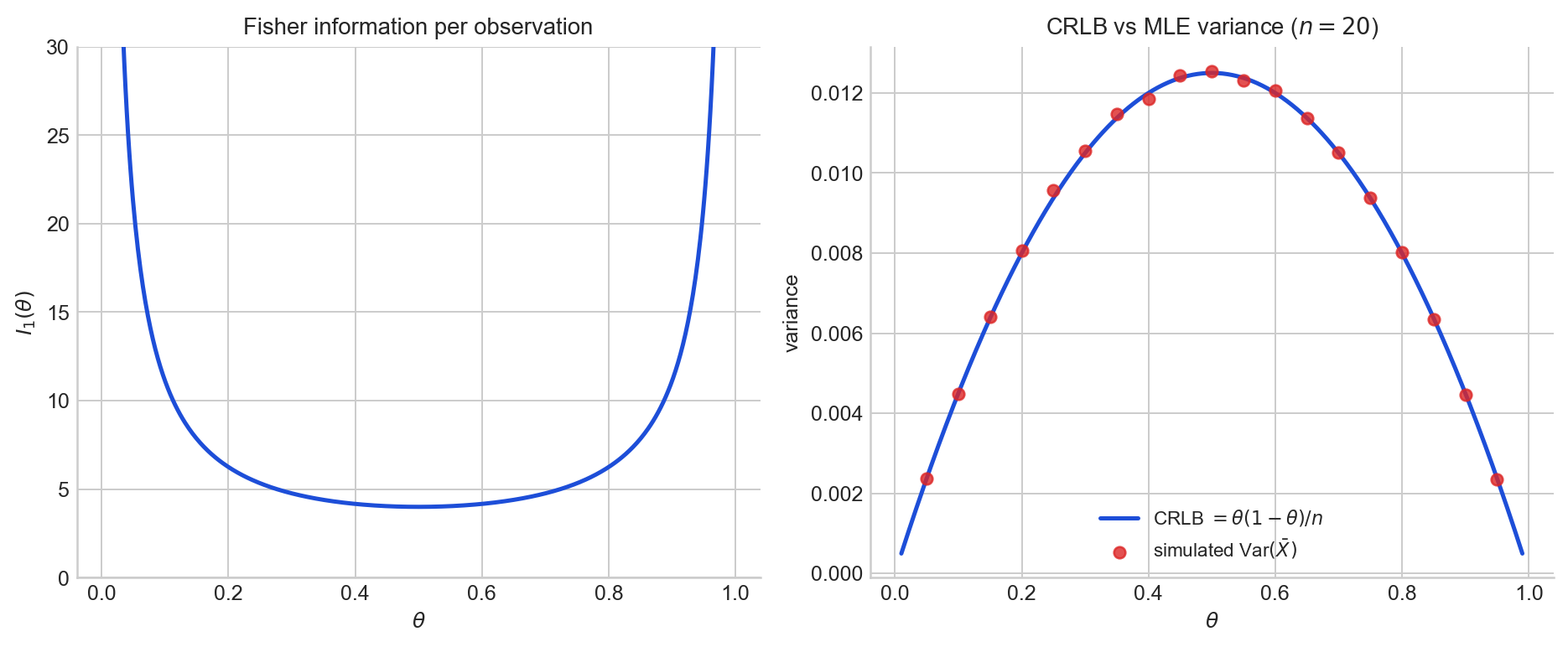
Figure 2. Left: Fisher information $I_1(\theta) = 1/[\theta(1-\theta)]$ for the Bernoulli model. Right: the Cramér–Rao lower bound on estimator variance (solid curve) and the simulated variance of the MLE $\bar{X}$ (dots) for $n = 20$.

Appendix

The proofs below follow the presentation in Rajen Shah, Principles of Statistics, Section 1.2.

A1: Equivalence of the two forms of Fisher information

We show that $I(\theta) = \mathbb{E}_\theta[S(\theta)^2] = -\mathbb{E}_\theta[\ell''(\theta)]$ in the scalar case.

Proof. Compute the second derivative of the log-density:

$$ \frac{\partial^2}{\partial\theta^2} \log f(x, \theta) = \frac{\frac{\partial^2}{\partial\theta^2} f(x, \theta)}{f(x, \theta)} - \left(\frac{\frac{\partial}{\partial\theta} f(x, \theta)}{f(x, \theta)}\right)^2. $$

Under regularity conditions, interchanging differentiation and integration gives

$$ \int \frac{\partial^2}{\partial\theta^2} f(x, \theta)\, dx = \frac{\partial^2}{\partial\theta^2} \int f(x, \theta)\, dx = 0, $$

so the expectation of the first term vanishes. Therefore

$$ -\mathbb{E}_\theta\!\left[\frac{\partial^2}{\partial\theta^2} \log f(X, \theta)\right] = \mathbb{E}_\theta\!\left[\left(\frac{\partial}{\partial\theta} \log f(X, \theta)\right)^2\right] = I(\theta). \quad\square $$

A2: Additivity under i.i.d. sampling

Proof. For i.i.d. data $X_1, \dots, X_n \sim f(\cdot, \theta)$, the score is $S_n(\theta) = \sum_{i=1}^n \nabla_\theta \log f(X_i, \theta)$. The Fisher information matrix is

$$ I_n(\theta) = \mathbb{E}_\theta[S_n(\theta)\, S_n(\theta)^\top] = \sum_{i=1}^n \sum_{j=1}^n \mathbb{E}_\theta\!\left[\nabla_\theta \log f(X_i, \theta) \cdot \nabla_\theta \log f(X_j, \theta)^\top\right]. $$

The terms $\nabla_\theta \log f(X_i, \theta)$ are i.i.d. and mean-zero, so the cross terms ($i \neq j$) vanish:

$$ I_n(\theta) = \sum_{i=1}^n \mathbb{E}_\theta\!\left[\nabla_\theta \log f(X_i, \theta) \cdot \nabla_\theta \log f(X_i, \theta)^\top\right] = n\, I_1(\theta). \quad\square $$

A3: Proof of the scalar Cramér–Rao lower bound

The key ingredient is the following lemma, which holds under regularity conditions allowing interchange of differentiation and integration.

Lemma. For any function $g$ of the data, $\mathbb{E}_\theta[S(\theta)\, g(X)] = \frac{\partial}{\partial\theta} \mathbb{E}_\theta[g(X)]$.

Proof of lemma. We have $\mathbb{E}_\theta[S(\theta)\, g(X)] = \int \frac{\partial}{\partial\theta} \log f(x, \theta) \cdot g(x) \cdot f(x, \theta)\, dx = \int \frac{\partial}{\partial\theta} f(x, \theta) \cdot g(x)\, dx = \frac{\partial}{\partial\theta} \int f(x, \theta) \cdot g(x)\, dx = \frac{\partial}{\partial\theta} \mathbb{E}_\theta[g(X)]$. $\square$

Proof of the CRLB. Let $\hat\varphi$ be any estimator. Apply the lemma with $g(X) = \hat\varphi(X)$:

$$ \text{Cov}_\theta(S(\theta),\, \hat\varphi) = \mathbb{E}_\theta[S(\theta) \cdot \hat\varphi] = \frac{\partial}{\partial\theta} \mathbb{E}_\theta[\hat\varphi], $$

where the first equality uses $\mathbb{E}_\theta[S(\theta)] = 0$. By the Cauchy–Schwarz inequality,

$$ \left(\frac{\partial}{\partial\theta} \mathbb{E}_\theta[\hat\varphi]\right)^2 \leq \text{Var}_\theta(S(\theta)) \cdot \text{Var}_\theta(\hat\varphi) = I(\theta) \cdot \text{Var}_\theta(\hat\varphi). $$

Rearranging:

$$ \text{Var}_\theta(\hat\varphi) \geq \frac{\left(\frac{\partial}{\partial\theta} \mathbb{E}_\theta[\hat\varphi]\right)^2}{I(\theta)}. $$

If $\hat\varphi$ is unbiased for $g(\theta)$, then $\mathbb{E}_\theta[\hat\varphi] = g(\theta)$ and the bound becomes $\text{Var}_\theta(\hat\varphi) \geq (g'(\theta))^2 / I(\theta)$. Taking $g(\theta) = \theta$ gives $\text{Var}_\theta(\hat\theta) \geq 1/I(\theta)$. For $n$ i.i.d. observations, replace $I(\theta)$ with $I_n(\theta) = n\, I_1(\theta)$. $\square$

A4: Multivariate Cramér–Rao lower bound

Proof. Let $\hat\varphi$ estimate $\varphi(\theta) \in \mathbb{R}$ and write $b = \nabla_\theta \mathbb{E}_\theta[\hat\varphi]$. Let $v = I(\theta)^{-1/2} u$ for an arbitrary unit vector $u \in \mathbb{R}^p$. The multivariate version of the lemma gives

$$ v^\top b = v^\top \mathbb{E}_\theta[S(\theta)\, \hat\varphi] = \mathbb{E}_\theta\!\left[v^\top S(\theta) \cdot (\hat\varphi - \mathbb{E}_\theta[\hat\varphi])\right], $$

where the last step uses $\mathbb{E}_\theta[S(\theta)] = 0$. By Cauchy–Schwarz:

$$ (v^\top b)^2 \leq \mathbb{E}_\theta[(v^\top S(\theta))^2] \cdot \text{Var}_\theta(\hat\varphi) = v^\top I(\theta)\, v \cdot \text{Var}_\theta(\hat\varphi). $$

Substituting $v = I(\theta)^{-1/2} u$ gives $\text{Var}_\theta(\hat\varphi) \geq (b^\top I(\theta)^{-1/2} u)^2$. Maximising over unit vectors $u$ by choosing $u \propto I(\theta)^{-1/2} b$ yields $\text{Var}_\theta(\hat\varphi) \geq b^\top I(\theta)^{-1} b$.

For an unbiased estimator $\hat\theta$ of $\theta \in \mathbb{R}^p$, apply this with $\varphi(\theta) = v^\top \theta$ for arbitrary $v$. Then $b = v$ and $\hat\varphi = v^\top \hat\theta$, giving $v^\top \text{Cov}_\theta(\hat\theta)\, v \geq v^\top I(\theta)^{-1} v$ for all $v$. This means $\text{Cov}_\theta(\hat\theta) - I(\theta)^{-1}$ is positive semi-definite. $\square$

A5: Equality condition

Equality in the Cauchy–Schwarz step of A3 holds if and only if $\hat\varphi - \mathbb{E}_\theta[\hat\varphi]$ is proportional to $S(\theta)$. In the scalar case with i.i.d. data and an unbiased estimator $\hat\theta$, this requires

$$ \hat\theta = \theta + \frac{1}{n\, I_1(\theta)} \cdot S_n(\theta) $$

for all $\theta$. This condition is quite restrictive and holds primarily for exponential family models with their natural sufficient statistics. When it does hold, the CRLB-achieving estimator is the unique UMVUE.

Sources

The material in this post draws on the likelihood inference chapter of the Principles of Statistics course at the University of Cambridge.

• Rajen Shah, Principles of Statistics, University of Cambridge lecture notes, Section 1.2.
• George Casella and Roger L. Berger, Statistical Inference, 2nd edition, Section 7.3.

The full code for all figures is in the Jupyter notebook on GitHub.