Stochastic convergence

When the objects we study are deterministic (e.g. real numbers, functions, sequences), convergence has an unambiguous meaning. We specify a notion of distance, and we ask whether the terms of a sequence eventually stay within any prescribed tolerance of a limit.

In statistics, however, the objects we work with are random. An estimator like $\bar X_n$ produces a different value each time we repeat the experiment. So when we write

$$ \bar X_n \to \mu, $$

the deterministic definition no longer applies directly: there is no single sequence of numbers to check against the limit. Instead, for each sample size $n$, $\bar X_n$ has a distribution, and for each realisation of the data, $\bar X_n$ traces out a different path.

This means there are genuinely different ways to ask whether a sequence of random variables “converges.” This post gives an intuitive explanation of three of them:

• convergence in distribution;
• convergence in probability;
• almost sure convergence.

Convergence for deterministic sequences

A sequence of real numbers $(x_n)$ converges to a limit $x$ if, for every $\varepsilon > 0$, there exists $N \in \mathbb{N}$ such that

$$ n \geq N \implies |x_n - x| < \varepsilon. $$

The definition asks for something specific: after some finite index, every subsequent term lies within $\varepsilon$ of the limit, no matter how small $\varepsilon$ is chosen. The sequence does not merely visit the neighbourhood of $x$; it enters and remains there permanently.

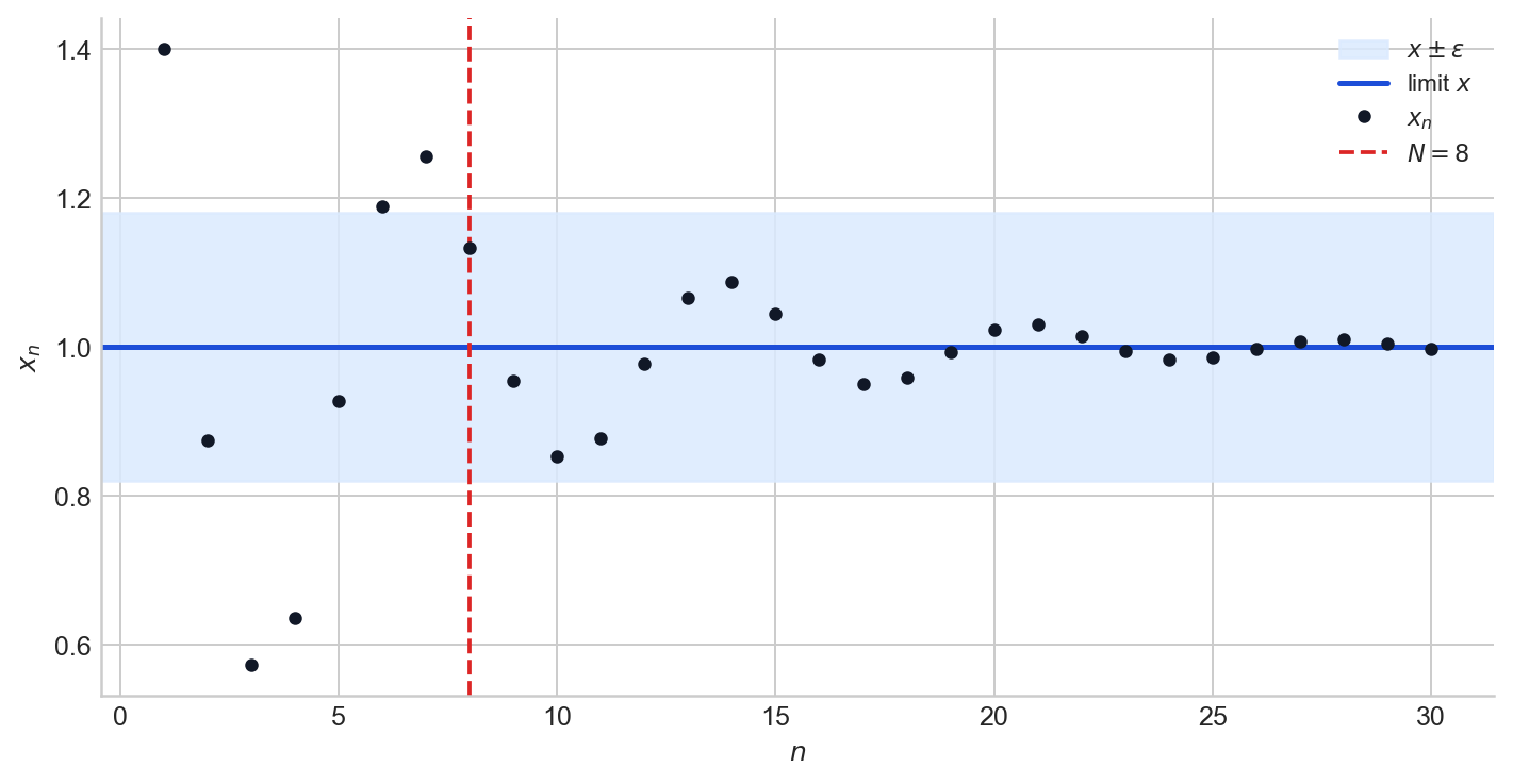
Figure 1. A convergent sequence and an $\varepsilon$-band around its limit. The red dashed line marks the index $N$ beyond which all terms stay inside the band.

Pointwise and uniform convergence for functions

Even in deterministic analysis, there is more than one notion of convergence. Consider a sequence of functions $f_n : [0,1] \to \mathbb{R}$.

Pointwise convergence says that for each fixed $x \in [0,1]$, the numerical sequence $f_n(x)$ converges. The rate at which $f_n(x)$ approaches its limit may depend on $x$, and in particular the index $N$ required to achieve a given tolerance $\varepsilon$ can vary across the domain.

Uniform convergence is stronger: it asks for a single $N$ that works simultaneously for all $x$. Formally, $f_n \to f$ uniformly on $[0,1]$ if

$$ \forall\, \varepsilon > 0,\;\exists\, N \in \mathbb{N} \text{ such that } n \geq N \implies \sup_{x \in [0,1]} |f_n(x) - f(x)| < \varepsilon. $$

The difference matters because pointwise convergence can fail to preserve basic properties of functions (continuity, integrability, interchange of limits) that uniform convergence does preserve.

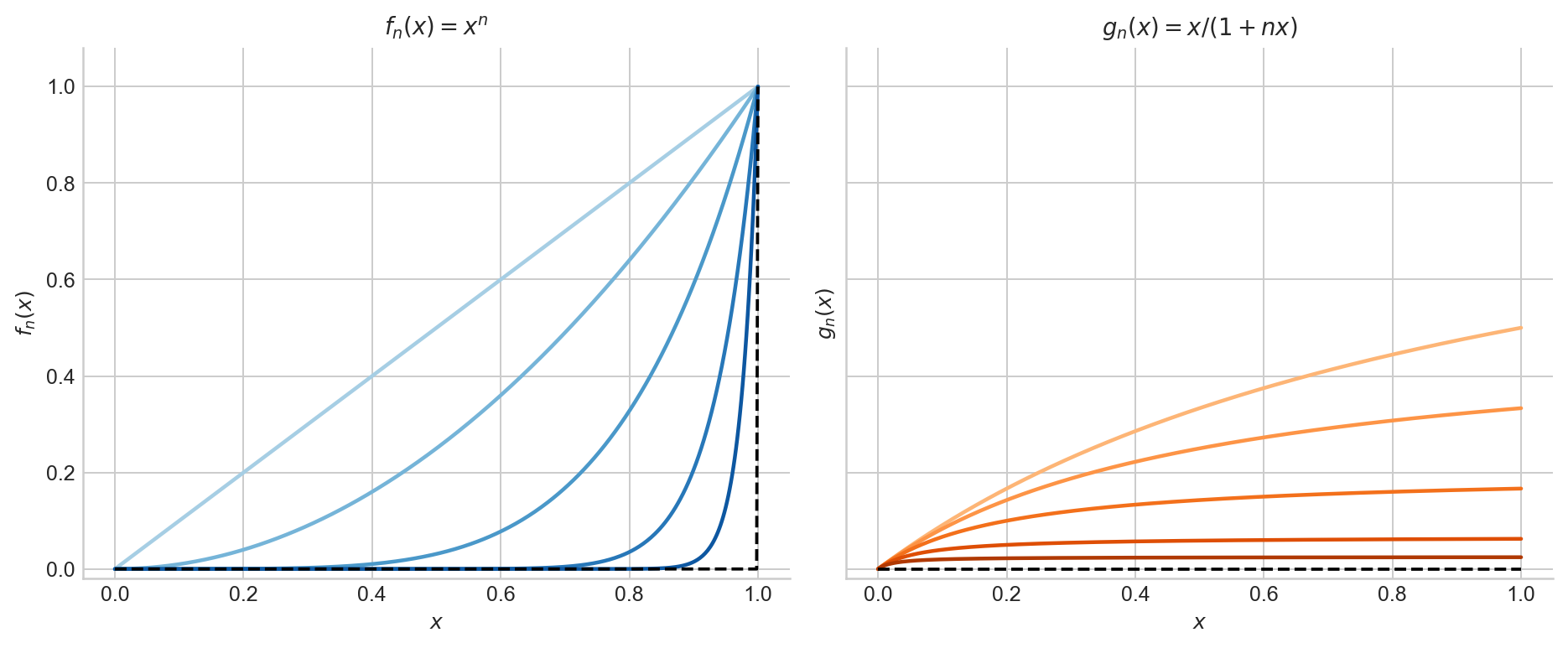
Figure 2. Left: $f_n(x) = x^n$ converges pointwise to $0$ on $[0,1)$, but $\sup_x |f_n(x) - f(x)| = 1$ for every $n$, so the convergence is not uniform. Right: $g_n(x) = x/(1+nx)$ converges uniformly to $0$, since $\sup_x g_n(x) = 1/(1+n) \to 0$.

Random variables as functions

Formally, a random variable is a measurable function $X : \Omega \to \mathbb{R}$, where $(\Omega, \mathcal{F}, \mathbb{P})$ is a probability space. The sample space $\Omega$ indexes all possible outcomes of an experiment; the randomness of $X$ comes entirely from the randomness of the outcome $\omega \in \Omega$. Once $\omega$ is determined, $X(\omega)$ is just a real number.

A sequence of random variables $(X_1, X_2, \ldots)$ is therefore a sequence of such functions, all defined on the same probability space. This gives rise to two fundamentally different ways of examining the sequence.

Pathwise view. Fix an outcome $\omega \in \Omega$. Then $X_1(\omega), X_2(\omega), \ldots$ is an ordinary numerical sequence, one specific realisation of the process. Different choices of $\omega$ produce different sequences.

Distributional view. Fix an index $n$. Then $X_n$ is a single random variable with its own distribution. As $n$ varies, we obtain a sequence of distributions.

These two views are why multiple notions of convergence arise. We can ask whether the distributions of $X_n$ approach a limiting distribution, whether the probability that $X_n$ deviates from a target vanishes, or whether the realised sequences $X_n(\omega)$ converge for almost every $\omega$. Each question leads to a different definition.

To make this concrete, consider the running average $\bar X_n = \frac{1}{n}\sum_{i=1}^n X_i$ of i.i.d. $N(0,1)$ draws. Figure 3 shows the same process from both angles: sample paths on the left, the distribution at a single fixed $n$ on the right.

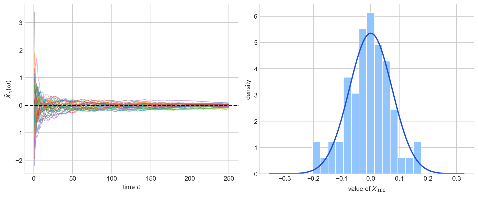
Figure 3. Left: sample paths of the running average $\bar X_n$ for i.i.d. $N(0,1)$ draws. Each path corresponds to a different $\omega$. Right: the empirical distribution of $\bar X_n$ at $n = 180$, with the $N(0, 1/180)$ density overlaid. The left panel is the pathwise view; the right panel is the distributional view.

Convergence in distribution

Recall that the distribution (or law) of a random variable $X$ is the probability measure $P_X$ on $\mathbb{R}$ defined by $P_X(B) = \mathbb{P}(X \in B)$. It is completely determined by the distribution function $F_X(t) = \mathbb{P}(X \leq t)$.

We write $X_n \to_d X$ if the distribution functions converge pointwise at every continuity point of $F_X$:

$$ F_{X_n}(t) \to F_X(t) \quad \text{for all } t \text{ at which } F_X \text{ is continuous.} $$

This is the weakest notion in the hierarchy. It is a statement purely about the sequence of distributions $P_{X_1}, P_{X_2}, \ldots$ and says nothing about whether the random variables $X_n$ and $X$ are close in any realisation. In particular, $X_n$ and $X$ need not even be defined on the same probability space.

When the limiting distribution is continuous, convergence in distribution implies that probabilities of intervals converge:

$$ \mathbb P(X_n \in [a,b]) \to \mathbb P(X \in [a,b]). $$

Figure 4 shows a sequence of normal densities $N(0, 1 + 1/n)$ approaching the $N(0,1)$ density as $n$ grows.

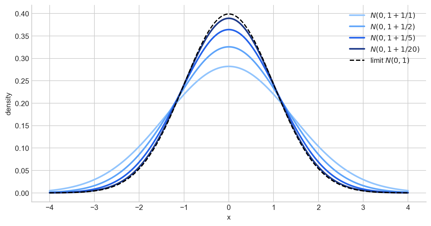
Figure 4. Densities of $N(0, 1 + 1/n)$ for several values of $n$, approaching the $N(0,1)$ limit (dashed).

The Central Limit Theorem

The CLT is the canonical example of convergence in distribution.

The CLT does not say that the centred-and-scaled statistic converges to a constant. It says its distribution approaches a Gaussian law. This is why convergence in distribution is the language of asymptotic normality, confidence intervals, and tests. A proof sketch is given in A2.

Figure 5 illustrates this with $\text{Exp}(1)$ samples: as $n$ increases, the histogram of $\sqrt{n}(\bar X_n - 1)$ approaches the standard normal density.

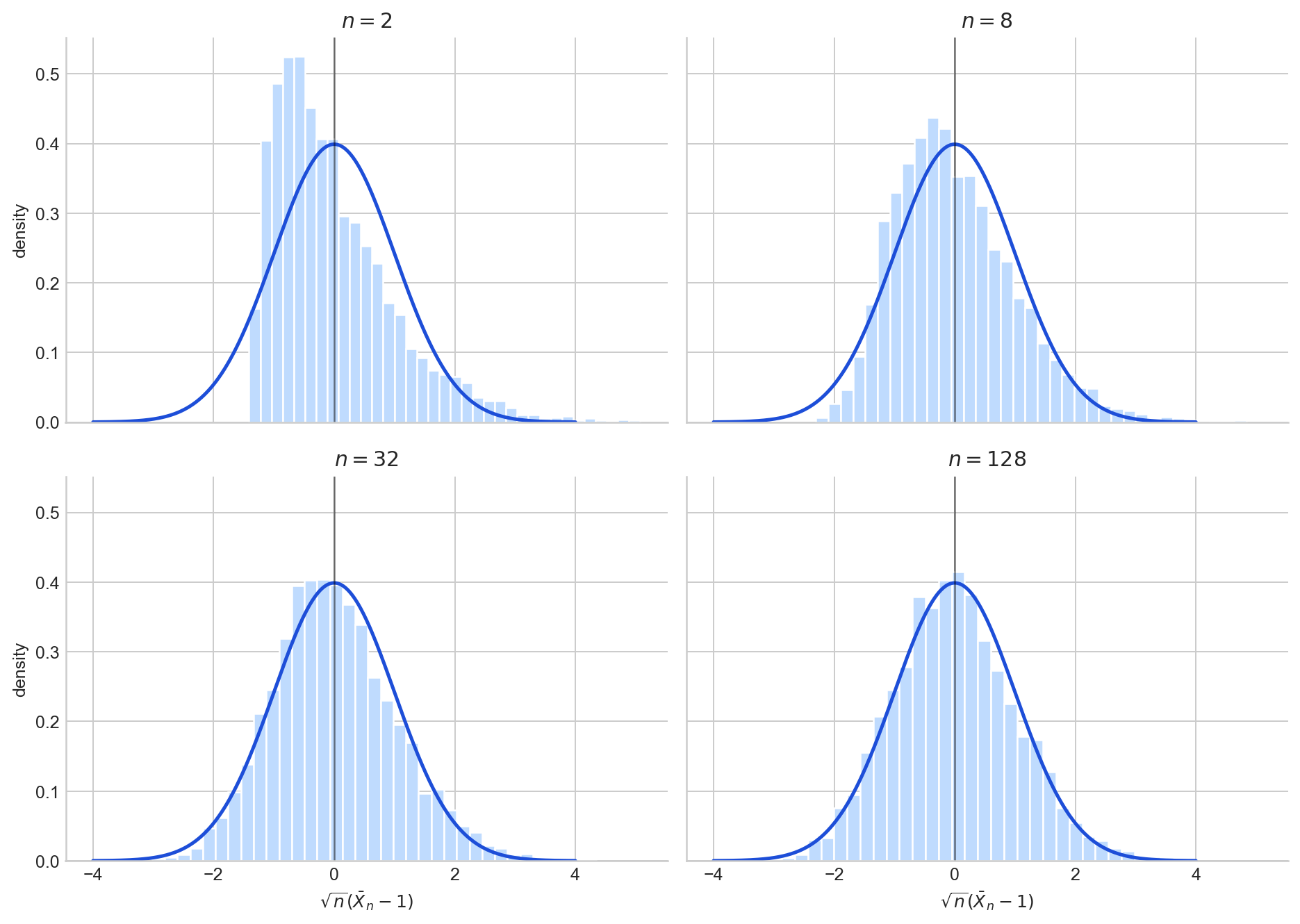
Figure 5. Histograms of $\sqrt{n}(\bar X_n - 1)$ for i.i.d. $\text{Exp}(1)$ draws at $n = 2, 8, 32, 128$, overlaid with the $N(0,1)$ density.

However, convergence in distribution does not say that $X_n$ is likely to be close to $X$ in any realisation. To make that kind of statement, we need a stronger notion.

Convergence in probability

Convergence in distribution only constrains the shape of the distribution of $X_n$. It does not require $X_n$ and $X$ to be defined on the same probability space, and says nothing about whether the values $X_n(\omega)$ are close to $X(\omega)$ for any particular outcome $\omega$. Convergence in probability fills this gap: it asks whether $X_n$ is close to $X$ as a random variable, not just in law. This requires both to live on the same $(\Omega, \mathcal{F}, \mathbb{P})$, because the expression $|X_n - X|$ must be well-defined.

We write $X_n \to_p X$ if for every $\varepsilon > 0$,

$$ \mathbb P(|X_n - X| > \varepsilon) \to 0. $$

The definition is a statement about each fixed $n$ separately. For a given $n$, consider the set of outcomes where $X_n$ is more than $\varepsilon$ from $X$:

$$ A_n(\varepsilon) = \{\omega \in \Omega : |X_n(\omega) - X(\omega)| > \varepsilon\}. $$

Convergence in probability says that for every $\varepsilon > 0$,

$$ \mathbb{P}(A_n(\varepsilon)) \to 0 \quad \text{as } n \to \infty. $$

Note that the bad set $A_n(\varepsilon)$ is allowed to change with $n$: the outcomes $\omega$ in $A_n(\varepsilon)$, corresponding to the paths that fall outside the $\varepsilon$-band at time $n$, need not be the same across different times. All that matters is that the total probability of this set shrinks.

Geometrically, this has a clean interpretation. Suppose we simulate $M$ independent copies of the entire experiment, producing $M$ sample paths $X_1(\omega_j), X_2(\omega_j), \ldots$ for $j = 1, \ldots, M$. Plot all $M$ paths on a single figure, draw an $\varepsilon$-band around the target $X$, and then draw a vertical line at time $n$. The cross-section at that vertical line consists of $M$ points, one per path. The proportion of those points that fall outside the $\varepsilon$-band is

$$ \hat p_n = \frac{1}{M}\sum_{j=1}^{M} \mathbf{1}\{|X_n(\omega_j) - X(\omega_j)| > \varepsilon\}, $$

which, by the law of large numbers, approximates $\mathbb{P}(|X_n - X| > \varepsilon)$ for large $M$. Convergence in probability says $\hat p_n \to 0$ as $n \to \infty$.

Figure 6 shows this for running averages of i.i.d. $N(0,1)$ draws with $\varepsilon = 0.12$.

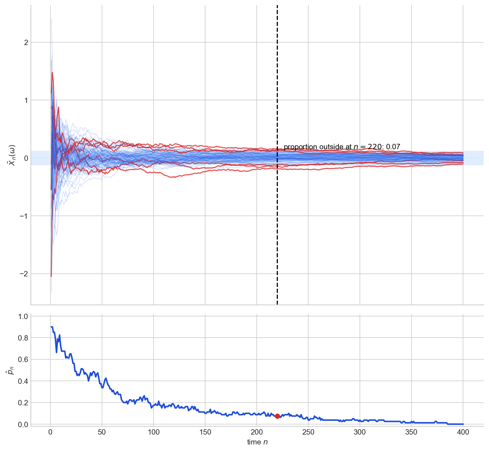
Figure 6. Top: sample paths of $\bar X_n$, with paths outside the $\varepsilon$-band at the dashed vertical line highlighted in red. Bottom: the estimated proportion $\hat p_n$ of paths outside the band, decreasing toward $0$.

The Weak Law of Large Numbers

The WLLN is the canonical example: it states that the sample mean converges in probability to the population mean.

The WLLN says that for large $n$, the sample mean is likely to be close to $\mu$: it is a per-$n$ guarantee that the probability of $\bar X_n$ being far from $\mu$ is small. It does not say that any particular realised sequence of running averages stays close permanently. The proof is a direct application of Markov’s inequality and is given in A1.

Figure 7 shows many running averages of i.i.d. Bernoulli$(1/2)$ draws concentrating around $1/2$.

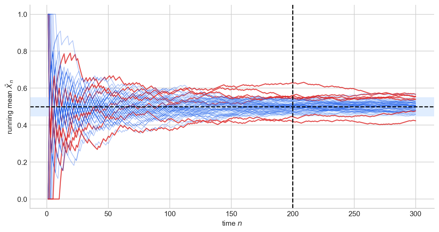
Figure 7. Running averages of i.i.d. Bernoulli$(1/2)$ draws, with paths outside the $\varepsilon$-band at the dashed vertical line highlighted in red. At large $n$, most paths concentrate near $\mu = 1/2$.

Convergence in probability is a per-snapshot property. At each fixed time $n$, the probability mass concentrates inside the $\varepsilon$-band: the density of $X_n$ piles up near $X$, and the tails thin out. But this is a statement about each time-slice separately; it says nothing about what happens along a single path over time. A specific path could leave the band at time $n_1$, return, leave again at $n_2$, and so on. As long as the mass outside the band at any single time goes to zero, convergence in probability is satisfied. Whether individual paths eventually settle down permanently is a strictly stronger requirement, addressed in the next section.

Almost sure convergence

Convergence in probability asks: at time $n$, is most of the probability mass near $X$? Almost sure convergence asks something much stronger: does each individual path $X_n(\omega)$ eventually settle down to $X(\omega)$?

We write $X_n \to_{a.s.} X$ if

$$ \mathbb P\bigl(\{\omega : X_n(\omega) \to X(\omega)\}\bigr) = 1. $$

To unpack this, consider the set

$$ \mathcal{G} = \{\omega \in \Omega : X_n(\omega) \to X(\omega)\}. $$

This is the set of all outcomes $\omega$ for which the realised sequence $X_1(\omega), X_2(\omega), \ldots$ converges to $X(\omega)$ in the ordinary deterministic sense. Its complement $\mathcal{N} = \Omega \setminus \mathcal{G}$ is the set of “bad” outcomes, those where the path fails to converge. Almost sure convergence says that $\mathcal{G}$ has full measure: $\mathbb{P}(\mathcal{G}) = 1$, or equivalently $\mathbb{P}(\mathcal{N}) = 0$. The bad set need not be empty, but it must be negligible under $\mathbb{P}$.

What does convergence of a single path actually require? For a fixed $\omega \in \mathcal{G}$ and any $\varepsilon > 0$, there must exist an index $N(\omega, \varepsilon)$ such that

$$ n \geq N(\omega, \varepsilon) \implies |X_n(\omega) - X(\omega)| < \varepsilon. $$

This is exactly the deterministic $\varepsilon$-$N$ definition from the first section, applied to the numerical sequence $X_1(\omega), X_2(\omega), \ldots$ The index $N$ depends on $\omega$: different realisations may take longer to settle down. But for almost every $\omega$, settlement does eventually happen: the path enters the $\varepsilon$-band and never leaves.

The Strong Law of Large Numbers

The SLLN says that with probability one, the realised running average enters every $\varepsilon$-band around $\mu$ and remains there. Note that the SLLN requires only a finite first moment, whereas the WLLN (as stated above) assumes a finite variance, which is a stronger condition. Figure 8 shows a single sample path of $S_n/n$ for a symmetric random walk, illustrating the eventual permanent entry into the band.

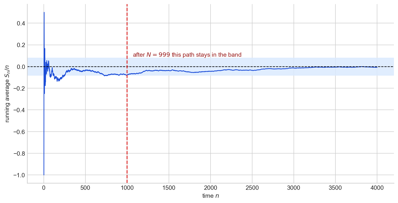
Figure 8. A single running average $S_n/n$ for i.i.d. $\pm 1$ draws. After the red dashed line, the path remains inside the $\varepsilon$-band permanently.

Convergence in probability vs almost surely

Both notions say that $X_n$ gets close to $X$, but they quantify “getting close” in fundamentally different ways. The cleanest way to see the distinction is through the language of failures.

Fix $\varepsilon > 0$ and say that a failure occurs at time $n$ if $|X_n(\omega) - X(\omega)| > \varepsilon$. Both convergence in probability and almost sure convergence imply that failures become rare, but they differ in how:

• Convergence in probability: for each fixed $n$, $\mathbb{P}(\text{failure at } n) \to 0$. At any single time, the proportion of paths outside the band is small.
• Almost sure convergence: for almost every $\omega$, there are only finitely many failures. Each individual path eventually stops leaving the band.

The first is a statement about vertical cross-sections: freeze time and ask how much mass lies outside the band. The second is a statement about horizontal trajectories: follow a single path and ask whether it ever leaves the band again.

A counterexample: convergence in probability without almost sure convergence

Let $(X_n)$ be independent with $\mathbb{P}(X_n = 1) = 1/n$ and $\mathbb{P}(X_n = 0) = 1 - 1/n$. Since $\mathbb{P}(|X_n| > \varepsilon) = 1/n \to 0$ for any $\varepsilon \in (0, 1]$, we have $X_n \to_p 0$.

But does each path eventually stay at $0$? The probability of a spike at time $n$ is $1/n$, and the sum $\sum_{n=1}^{\infty} 1/n = \infty$ diverges. By the second Borel–Cantelli lemma (which applies because the $X_n$ are independent), with probability $1$ infinitely many of the events $\{X_n = 1\}$ occur. Every path keeps producing spikes; they become sparser, but they never stop. So $X_n \not\to_{a.s.} 0$.

The key is the difference between “each individual failure becomes unlikely” and “the total number of failures is finite.” Convergence in probability gives the first; almost sure convergence requires the second. The Borel–Cantelli lemma makes the gap precise: if the failure probabilities $p_n = \mathbb{P}(|X_n| > \varepsilon)$ satisfy $\sum p_n < \infty$, then almost sure convergence holds (first Borel–Cantelli). If $\sum p_n = \infty$ and the events are independent, then almost sure convergence fails (second Borel–Cantelli).

The hierarchy

The three notions form a strict implication chain:

$$ X_n \to_{a.s.} X \implies X_n \to_p X \implies X_n \to_d X. $$

Neither reverse implication holds in general, as the counterexamples above demonstrate. The level of guarantee weakens as we move down: almost sure convergence controls paths, convergence in probability controls mass at each fixed time, and convergence in distribution controls only the law. A proof of both implications is given in A3.

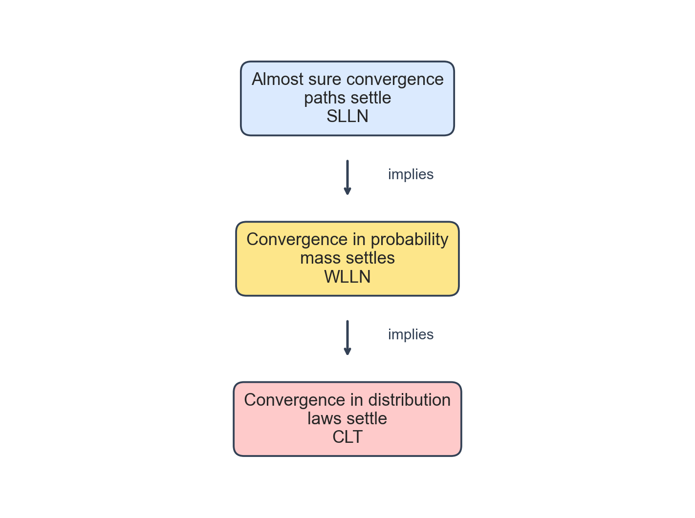
Figure 9. The implication hierarchy, with the associated flagship theorem at each level.

Working with convergence

Up to now, we have been asking what the different notions of convergence mean. In practice, though, asymptotic statistics is not built by proving every convergence from scratch. One establishes a small number of foundational results, the WLLN, the CLT, consistency of a particular estimator, and then uses a handful of general theorems to assemble more complex conclusions. This is where the subject starts to feel like ordinary analysis again: a toolkit of rules for passing limits through operations.

Joint convergence

The first question is whether convergence of two sequences separately implies convergence of the pair. For convergence in probability and almost sure convergence, the answer is as clean as one could hope.

Intuitively, controlling each coordinate separately is enough to control the whole vector, because closeness in $\mathbb{R}^{d+k}$ is just closeness in each coordinate simultaneously.

This matters constantly in practice. If one has separately established that $\bar X_n \to_p \mu$ and $\hat\sigma_n^2 \to_p \sigma^2$, the theorem immediately gives $(\bar X_n, \hat\sigma_n^2) \to_p (\mu, \sigma^2)$, putting both limits in a form that continuous functions can act on.

Convergence in distribution is more delicate. Knowing $X_n \to_d X$ and $Y_n \to_d Y$ separately says nothing about how the pair $(X_n, Y_n)$ behaves jointly, because distributional convergence controls marginals but not dependence structure. There is, however, one important special case: if one of the limits is a constant $c \in \mathbb{R}^k$, then

$$ (X_n, Y_n) \to_d (X, c) \iff X_n \to_d X \text{ and } Y_n \to_p c. $$

This pattern, one sequence with a non-degenerate limiting distribution and another converging in probability to a fixed constant, is exactly the setting of Slutsky’s lemma.

The Continuous Mapping Theorem

Once one has a convergence in hand, the next question is whether applying a function to both sides preserves it. The answer is yes, as long as the function is continuous.

This is the stochastic analogue of the familiar fact that continuous functions preserve limits. For example, $X_n \to_p X$ implies $X_n^2 \to_p X^2$, $\exp(X_n) \to_p \exp(X)$, and $\sin(X_n) \to_p \sin(X)$; the same holds for convergence in distribution and almost sure convergence. Continuous transformations do not destroy asymptotic information: once a convergence is established, it propagates through any continuous operation.

Slutsky’s Lemma

Combining joint convergence and the continuous mapping theorem in the distributional setting gives what is perhaps the most-used result in asymptotic statistics.

The logic is simple: because $Y_n \to_p c$, it behaves asymptotically as though it were already the constant $c$, so one may substitute $c$ for $Y_n$ inside any continuous expression in the limit.

The canonical illustration is standardisation. Suppose the CLT gives $\sqrt{n}(\bar X_n - \mu) \to_d N(0, \sigma^2)$, and suppose $\hat\sigma_n \to_p \sigma$ (which follows from the WLLN applied to the sample variance). Slutsky’s lemma then gives

$$ \frac{\sqrt{n}(\bar X_n - \mu)}{\hat\sigma_n} \to_d N(0, 1). $$

This mechanism underlies many asymptotic pivots in classical statistics.

Passing to expectations: Dominated Convergence

The results so far concern the convergence of random variables themselves. A separate question is whether convergence of $W_n$ to $W$ implies $\mathbb{E}(W_n) \to \mathbb{E}(W)$. In general it does not: mass can drift into rare but large values, making the expectations diverge even as the random variables converge. A standard sufficient condition rules this out.

The condition is that all terms in the sequence are dominated pointwise by a single integrable envelope. When this holds, the tails cannot escape to infinity, and expectation behaves continuously with respect to convergence.

A representative application is in likelihood theory. To establish continuity of the population log-likelihood $\theta \mapsto \mathbb{E}_{\theta_0} \log f(X, \theta)$, one shows that $\log f(X, \theta_n) \to \log f(X, \theta)$ pointwise as $\theta_n \to \theta$, and then uses dominated convergence to pass the limit through the expectation.

Appendix

The proofs below follow the presentation in Rajen Shah, Principles of Statistics, Sections 1.3–1.4.

A1: Weak Law of Large Numbers

We use Markov’s inequality: if $Z \geq 0$ then $\mathbb{P}(Z \geq t) \leq t^{-1}\mathbb{E}(Z)$.

Proof. Apply Markov’s inequality to $(\bar X_n - \mu)^2$:

$$ \mathbb{P}(|\bar X_n - \mu| > \varepsilon) = \mathbb{P}\bigl((\bar X_n - \mu)^2 > \varepsilon^2\bigr) \leq \frac{\mathbb{E}(\bar X_n - \mu)^2}{\varepsilon^2} = \frac{\text{Var}(\bar X_n)}{\varepsilon^2} = \frac{\text{Var}(X_1)}{n\varepsilon^2} \to 0 $$

as $n \to \infty$. $\square$

A2: Central Limit Theorem

The standard proof uses characteristic functions. We sketch the argument in the univariate case.

Proof. Write $Z_i = (X_i - \mu)/\sigma$ so that $\mathbb{E}(Z_i) = 0$ and $\text{Var}(Z_i) = 1$. The characteristic function of $Z_i$ satisfies

$$ \varphi_Z(t) = \mathbb{E}(e^{itZ_1}) = 1 - \frac{t^2}{2} + o(t^2) $$

as $t \to 0$, using the expansion $e^{itZ_1} = 1 + itZ_1 - t^2Z_1^2/2 + \cdots$ and taking expectations. The quantity we want to study is $S_n = \frac{1}{\sqrt{n}}\sum_{i=1}^n Z_i$, whose characteristic function is

$$ \varphi_{S_n}(t) = \bigl[\varphi_Z(t/\sqrt{n})\bigr]^n = \Bigl[1 - \frac{t^2}{2n} + o(t^2/n)\Bigr]^n \to e^{-t^2/2} $$

as $n \to \infty$. Since $e^{-t^2/2}$ is the characteristic function of $N(0,1)$, Lévy’s continuity theorem gives $S_n \to_d N(0,1)$, which is equivalent to $\sqrt{n}(\bar X_n - \mu) \to_d N(0, \sigma^2)$. $\square$

A3: The hierarchy

We prove both implications in the chain $X_n \to_{a.s.} X \implies X_n \to_p X \implies X_n \to_d X$.

Almost sure convergence implies convergence in probability. Fix $\varepsilon > 0$ and define $B_n = \{\sup_{k \geq n} |X_k - X| > \varepsilon\}$. The sets $B_n$ are decreasing in $n$, and $\bigcap_n B_n \subseteq \{\omega : X_n(\omega) \not\to X(\omega)\}$, which has probability zero by assumption. Continuity of measure gives $\mathbb{P}(B_n) \to 0$. Since $\{|X_n - X| > \varepsilon\} \subseteq B_n$, we conclude $\mathbb{P}(|X_n - X| > \varepsilon) \to 0$. $\square$

Convergence in probability implies convergence in distribution. Let $t$ be a continuity point of $F_X$ and fix $\varepsilon > 0$. Since $\{X_n \leq t\} \subseteq \{X \leq t + \varepsilon\} \cup \{|X_n - X| > \varepsilon\}$, we have

$$ F_{X_n}(t) \leq F_X(t + \varepsilon) + \mathbb{P}(|X_n - X| > \varepsilon). $$

Similarly, $\{X \leq t - \varepsilon\} \subseteq \{X_n \leq t\} \cup \{|X_n - X| > \varepsilon\}$ gives

$$ F_X(t - \varepsilon) - \mathbb{P}(|X_n - X| > \varepsilon) \leq F_{X_n}(t). $$

Letting $n \to \infty$ and using $\mathbb{P}(|X_n - X| > \varepsilon) \to 0$ yields $F_X(t - \varepsilon) \leq \liminf_n F_{X_n}(t) \leq \limsup_n F_{X_n}(t) \leq F_X(t + \varepsilon)$. Taking $\varepsilon \to 0$ at a continuity point of $F_X$ gives $F_{X_n}(t) \to F_X(t)$. $\square$

Sources

The material in this post is covered in the Principles of Statistics course at the University of Cambridge; the primary reference throughout is the accompanying lecture notes.

• Rajen Shah, Principles of Statistics, University of Cambridge lecture notes, Sections 1.3 and 1.4.
• Pierre Lafaye de Micheaux and Benoit Liquet, “Understanding Convergence Concepts: A Visual-Minded and Graphical Simulation-Based Approach”.
• Robby McKilliam and others, “Convergence in probability vs. almost sure convergence”.

The full code for all figures is in the Jupyter notebook on GitHub.